
For a full list of BASHing data blog posts see the index page. ![]()
Mapping with gnuplot, part 2
The first part of this series appeared back in 2018. It describes how you can use gnuplot to build a simplified GIS. I wasn't intending to do any more with this idea, but I was tinkering with animated map GIFs of Tasmania and realised that the gnuplot approach had some advantages. This post and the next one explain what I did. You don't need to refer to that 2018 post, since I'll repeat and update the information here.
Preparing data files for the base map. I started with two shapefiles for Tasmania. One was a polygon shapefile for the coastlines, the other a polyline shapefile for the main roads. I added both as layers in QGIS with EPSG:4326 as the project CRS. I then used the MMQGIS plugin to extract coordinates for the nodes with the "Geometry Export to CSV File" option. This option built two CSVs for each shapefile, one for the nodes and one for the associated attributes.
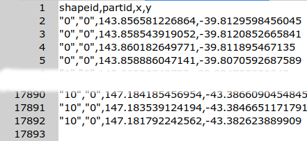
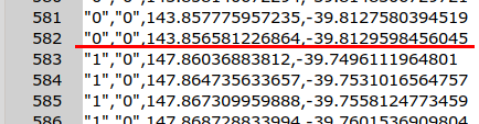
The nodes CSV was the relevant file in each case. Each node appeared in the CSV with four fields: a shape identifier ("shapeid"), a sub-shape identifier ("partid"), an x value (longitude) and a y value (latitude). The coastline CSV, for example, had 17891 nodes divided among 11 shapes numbered from "0" to "10":
To get this file ready for gnuplot I needed to separate the lon/lat node lists for each of the 11 polygons, like this:
143.8578 -39.8128
143.8566 -39.8130
147.8604 -39.7496
147.8647 -39.7531
147.8673 -39.7558
For this job I used an AWK command on the CSV after tailing off the header line:
awk -F"," \
'NR==1 || $1==a {a=$1; printf("%0.4f %0.4f\n",$3,$4)}
$1 != a {printf("\n\n%0.4f %0.4f\n",$3,$4); a=$1}' demo
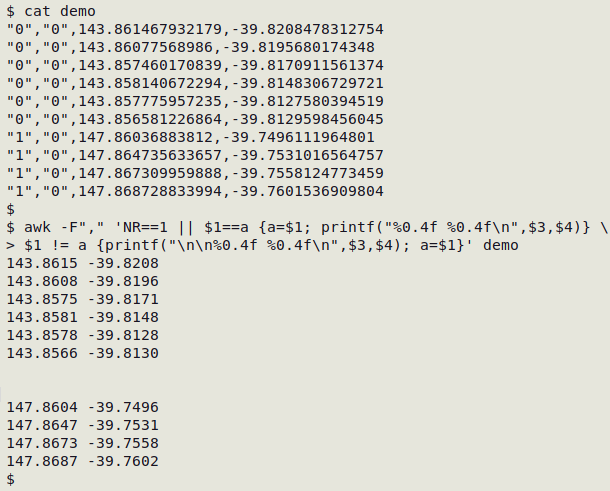
The coastline CSV was reduced to the 11-section list "tas3" of lons and lats, and the main roads CSV was converted similarly to "roads3".
UPDATE 2024-02-13. Below is a much improved command for generating the plotting file from the raw "temp1-nodes.csv" exported by MMQGIS. The improved command allows for multiple partID shapes and also deletes duplicate coordinate pairs resulting from the rounding to four decimal places:
awk -F"," 'NR>1 {a[$1$2]=a[$1$2] RS $0} END {for (i in a) print a[i]}' temp1-nodes.csv | awk -F"," 'NR>1 {if ($0=="") print; else if (!b[$0]++) printf("%0.4f %0.4f\n",$3,$4)}' > tas3
For an explanation of this command, see the upcoming post "Mapping with gnuplot, part 4" in the second BASHing data series.
Building a base map. Below is a configuration file ("smallbase") similar to the one I used to create a base map with gnuplot. It differs from the real one only in having a smaller overall canvas size, so I could display it more easily in this blog post:
set terminal png size 620,620
set output "map.png"
set size ratio 1.1
set style line 1 lc rgb "gray" lw 0.5
set style line 2 lc rgb "black" lw 0.5
set format x "%0.1f"
set format y "%0.1f"
set xrange [143.5:149.0]
set yrange [-44.0:-39.5]
set xtics 0.5
set ytics 0.5
set tics nomirror out font "Sans, 8"
set grid linestyle 1
unset key
plot "tas3" with lines linestyle 2, \
"roads3" with lines linestyle 1
And here's the "map.png" built by the command "gnuplot smallbase":
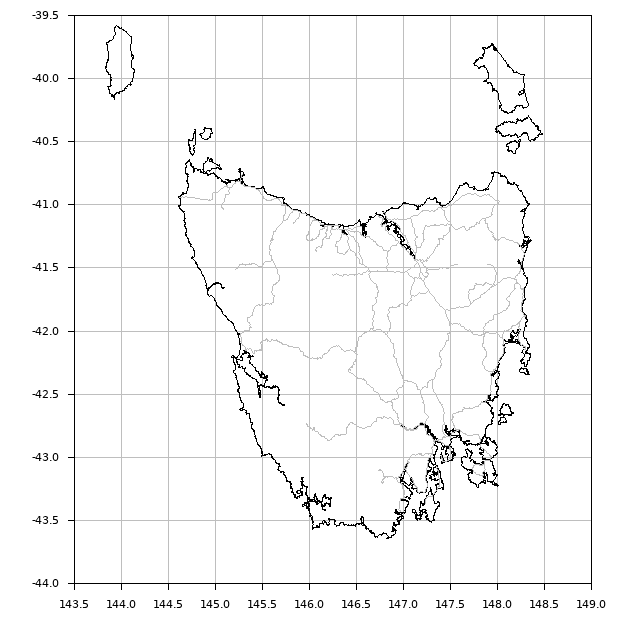
This might look like a Mercator projection, but it isn't. I've adjusted the width-height ratio of an equirectangular projection (set size ratio 1.1) so that the shape of Tasmania approximates its shape in a Mercator plot. Call it a "stretched-equirectangular projection"?
In the next post (6 April 2022) I show how I built my map animations, starting with this base map.
Last update: 2024-02-13
The blog posts on this website are licensed under a
Creative Commons Attribution-NonCommercial 4.0 International License